The 2005 Atlantic Hurricane Season and
Labour Market Transitions

Author: Edward Allenby

                                           Supervisor: Gianni De Fraja

This Dissertation is presented in part fulfilment of the requirement for the completion of an MSc in the School of Economics, University of Nottingham. This work is the sole responsibility of the candidate.

Abstract

The 2005 Atlantic hurricane season caused significant disruption to jobs and livelihoods across Alabama, Florida, Louisiana, Mississippi and Texas. Ag gregated employee-employer linked data is used to study how labour market
transition rates were impacted by this hurricane season. This paper finds that, as a result of the hurricanes, the job separation rate rose but only in the immediate aftermath of the storms. The hiring rate initially declined before
rising and remaining persistently elevated for five years. Job turnover is also shown to decrease in the wake of the storms. Counties with greater hurricane damage experienced larger changes in separation, hiring and turnover rates. No evidence of spillover effects for labour market transitions were found to be present in areas that neighbour damaged counties. The impact of the storms was heterogeneous across industrial sectors, significant losses were seen in the accommodation and leisure sector, whilst the construction sector saw a notable improvement in labour market transitions, however all sectors experienced a decline in job turnover.

1 Introduction

The 2005 Atlantic hurricane season saw 28 storms hit the US Gulf states, surpassing the previous record of 20, set in 1933 (National Oceanic and Atmospheric Administration, 2005). Within the season, there were a number of
Category 5 hurricanes such as hurricanes Emily, Katrina and Rita, which all made landfall in the third quarter of 2005. The most devastating of these was Hurricane Katrina which hit the US coastline on August 23, causing 1,800 deaths, over $100 billion in total losses and $34 billion in insured losses across Alabama, Louisiana, Florida and Mississippi (Blake et al. 2011). Later in the season, Hurricane Rita made landfall across Texas and Louisiana on September 24 and was the most intense hurricane ever recorded in the Gulf of Mexico and the fourth-most intense Atlantic hurricane (Knabb et al. 2006).

In response to the impact of these storms, the US Senate approved a $10.5 billion aid package on September 1, this was soon followed by President Bush requesting an additional $51.8 billion which was approved by Congress on September 8 (Deryugina et al. 2018). The significant amount of taxpayer money spent on disaster relief relating to the 2005 hurricane season highlights the importance of understanding the nuance behind which groups of workers were most affected, to ensure that the funding of future disaster relief packages are allocated effectively. As a result, the motivation behind this paper is to gain a better understanding of how job separation, hiring and turnover behaviour was impacted by the storm season. This can be beneficial in assisting future policymakers when creating targeted economic disaster responses due to this study seeking to explore questions such as which industries faced an increase in the probability of job separations and by how much, as well as, where government-supported hiring programs may be most effective.

This research utilises housing damage data from the Federal Emergency Management Agency (FEMA) and the Department for Housing and Urban Development (HUD) to identify the hurricane-affected counties. It is used alongside aggregated county-level employee-employer-linked worker microdata from the US Census Bureau and the Longitudinal Employer-Household Dynamics (LEHD) program, which provides information on labour market behaviour over time. A synthetic control methodology is employed to analyse how labour market transition
rates behaved in the aftermath of the hurricane season. The control groups are formed from a weighted average of counties in the five storm-hit states that were neither directly affected by the storms, nor nearby affected counties. The control groups are constructed using a matching process to ensure that the control group closely resembles the hurricane-affected counties across a variety of social, demographic and economic characteristics prior to the hurricane season, for each labour market transition rate of interest.

The main findings of this paper show that hurricane affected counties suffered a 3.7 percentage point rise in the average job separation rate, a 0.75 percentage point fall in the hiring rate and a fall of 1.75 percentage points in the turnover rate, in the immediate aftermath of the hurricanes in 2005 Q3. However, beyond 2005 Q3,
results show that the rise in separations has little persistence and diminishes by 2006 Q1, the hiring rate rebounds to almost two percentage points above its counterfactual and remains elevated for almost the entire post-storm sample and the turnover rate shows a marginally negative storm effect in most post-storm periods. These findings indicate that whilst job separations were immediate and severe, positive hiring effects lasted significantly longer, consistent with the wealth of previous research that show an increase in labour demand and earnings in the long-term after the storms. The combination of how these two transition rates
evolved influenced the turnover rate by increasing the proportion of the workforce
that were in fresh new jobs, thus lead to a subdued turnover rate in subsequent
periods.

This study also finds evidence that increasingly severe housing damage is associated with greater magnitudes of change to labour market transition rates, whilst counties experiencing relative minor damage are shown to have experienced insignificant storm effects. Our results suggest that there was no evidence of these storm effects
spilling over from damaged counties into neighbouring undamaged counties. Examining whether the impact of the storms on labour market transition rates differed by industrial sector shows that the construction sector was the primary beneficiary of the storms, seeing lower separation rates and greater hiring rates, meanwhile the accommodation and leisure sector was most negatively impacted, thus providing evidence for the importance of targeted disaster response programs.

The study of the longer-term impacts of the storm season on the behaviour of labour market transitions distinguishes this paper from much of the past labour market research on these storms, which primarily study the evolution of earnings and employment immediately after the storms across specific cities, geographies and groups of individuals. For example, a large number of studies focus on the employment and earnings impact on individuals in specific areas such as New Orleans (e.g. Dolfman et al. 2007), or cities in Texas that received a substantial number of evacuees (Clayton and Spletzer, 2006). Understandably, one of the core pillars of the labour market literature, studying the 2005 US storm season, is the experiences of evacuees. Here, authors have built on the findings within the job displacement literature that show evacuees separated from their jobs would experience a notable period of unemployment due to disrupted social networks and geographical relocation (Kletzer, 1998). Applying this to the 2005 Atlantic storm season, many researchers find similar results in that evacuees naturally experience worse outcomes than those who do not have to evacuate, which is linked to the
severity of damage faced. However, the evacuees who later return to their pre-storm residence, close the employment and earnings gap with non-evacuees after 1-3 years, whereas evacuees who do not return home and permanently relocate, fare far worse (Vigdor, 2007; Groen and Polivka, 2008; Zissimopoulos and Karoly, 2010; Sacerdote, 2012). Additionally, many influential papers study the labour market outcomes over a relatively short time horizon, normally between 12-24 months after the storms, where typically lower labour participation and greater wages are found. For example, Belasen and Polacheck (2008) study the hurricane effects on employment and earnings in Florida until 24 months after the storms and find that the employment rate fell by 4.8 percent whilst wages grew by 4.4 percent. However, there are two recent exceptions to this, that take advantage of the longer post-storm time series now available to analyse longer-term employment and earnings. Deryugina et al. (2018) study the tax returns from individuals residing in New Orleans up to eight years after the storms, whilst Groen et al. (2020) analyse the evolution of earnings across four states with a seven-year post-storm sample. Both find that the wages of hurricane-affected individuals grew relative to the control groups used. However, they disagree over the driving force of this result. Deryugina et al. (2018) argue that relative wage growth for affected individuals was mainly a result of higher living costs, Groen et al. (2020) instead decompose the higher wages into within job earnings changes and earnings changes as a result of job separations, and convincingly argue that local industry-specific changes in the supply and demand of labour was the primary driver of earnings growth.

This paper builds on a variety of research avenues present in the relevant literature. Firstly, like in Deryugina et al. (2018) and Groen et al. (2020), a five-year post-storm sample is used, which is considerably longer than many past studies, thus allowing for a more complete picture of post-storm labour market outcomes. Secondly, as stated earlier, the impact of the hurricane season on a specific state or city is often the focus of papers and few look at the causal impacts across all affected states and counties. Therefore, with Groen et al. (2020), this paper’s use of a larger research area provides a more geographically comprehensive set of results. However, this study does depart from the research of Groen et al. (2020) by examining the storms’ effect on job separation, hiring and turnover rates, rather than the impact on earnings and the employment rate. One of the key findings in Groen et al. (2020) provides part of the justification for this study’s focus on these variables, they found that 97 percent of the losses in earnings over the first year was a result of job separations rather than within employment earnings changes.

Therefore, beyond just the non-pecuniary costs individuals face when separated from their jobs, this also demonstrates the importance of job separations and hiring in determining the earnings of households. As a result, to gain a better understanding of earnings dynamics after natural disasters, to assist future policymaking, a thorough understanding of the extent to which different groups of individuals are exposed to job separations, hiring and worker turnover, is justified. The remainder of this paper is structured as follows. Section 2 describes the data used in the empirical analysis of this paper, with an emphasis on worker and damage data, as well as providing summary statistics. Second 3 explains the synthetic control methodology used. Section 4 presents the main findings of this paper, then looks at how the findings vary by damage severity and industrial
sector, and whether there is evidence of spillover effects.

2 Data

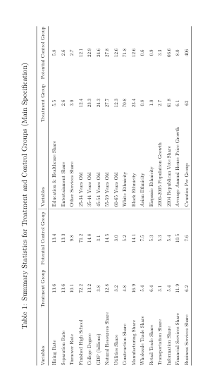
This section will outline the data used for county-level worker transitions, storm damage, predictor variables used in the matching process, and how the treatment and control groups are defined. Summary statistics will also be presented for all the variables used to construct the treatment and control group in this paper’s main
specification.

2.1 Worker Data

To study the behaviour of job separation, hiring and turnover rates over time, this paper uses the Quarterly Workforce Indicators produced by the US Census Bureau’s Center for Economic Studies as part of the Longitudinal Employer-Household Dynamics (LEHD) program. The QWI provide local labour market statistics by industry, worker demographics, employer age and size, across multiple levels of geography (e.g., national, state, county, metropolitan statistical area and individuals) (Abowd et al. 2006)1. The LEHD is a large longitudinal
micro database which covers 95 percent of US private sector jobs, constructed from an array of administrative records, demographic surveys, economic surveys and censuses.

This paper uses the public-access aggregated QWI data at the county level and at a quarterly frequency. Here, the three variables of interest are the job separation, hiring and turnover rates from 2001 Q3 to 2010 Q4. The job separation rate is the 1Whilst the QWI data can be cut by a variety of demographic and firm characteristics, this paper doesn’t choose to exploit this opportunity other than the industry analysis presented in Section 4.4, where the three variables of interest are collected across each county for each industry from 2001 Q3 to 2010 Q4. The opportunity for splitting the QWI data by demographic and firm characteristics is left to future research.

number of separations as a percentage of average employment, therefore providing the fraction of the workforce that are leaving their jobs in a given quarter. Similarly, the hiring rate is defined by the number of hires as percentage of employment, indicating the fraction of the workforce that are starting or returning to new jobs. The turnover rate is defined as the sum of hires and separations in a given quarter, divided by that quarter’s employment, thus shows the degree of labour market churn occurring. Whilst the job turnover rate often receives less focus than other labour market variables during economic shocks, its importance is demonstrated through its potential to show changes in the ability of labour markets to efficiently allocated workers to their most productive uses. These three variables are used in sections 3 and 4 as the outcomes of interest when analysing the impact of the hurricane season. As is discussed later in Section 2.3, the separation, hiring and turnover rates are collected across all 534 counties in Alabama, Florida, Louisiana, Mississippi and Texas in each of the 38 time periods of this study.

2.2 Damage Data

County-level information regarding the damage inflicted by the hurricanes is derived from storm damage assessments carried out by FEMA. This shows the number and percentage of housing units in a given county that received different levels of damage (HUD, 2006). FEMA groups the damage level of affected housing units into three tiers, minor, major and severe damage. A house is classed as having experienced minor damage if the property inspection finds damage of less than $5,200, majorly damaged houses are defined as receiving between $5,200 and less than $30,000 of damage, whereas a house is considered severely damaged if damages are in excess of $30,000. Combining this information with the number of housing units in each county, HUD provides statistics for the share of each counties’ housing units that received minor, major and severe damage as a result of the hurricanes. One factor to consider is the extent to which damage inflicted on an area’s housing units may partially reflect the relative wealth of that neighbourhood, given richer neighbourhoods may posses more extensive storm defences. Groen et al. (2020) identified this possible problem and used physical measures such as wind speed to establish the degree of damage. They found that damage was not sensitive to local storm defence efforts, thus this potential bias is not considered an area of concern.

2.3 Treatment and Control Groups

To study the impact of the 2005 hurricane season on labour market transitions, one must first outline which counties are considered affected by the hurricanes and which counties can be used as potential controls. In this paper’s main specification, outlined in Section 4.1, we follow Groen et al. (2020) in defining the treatment group as any county where 1% or more of housing units were classed as receiving severe or major storm damage. As a result, the treatment group consists of 63 counties across Alabama, Florida, Louisiana, Mississippi and Texas. Later, in Section 4.2, we relax this definition of the treatment group to study the extent to which the changes in labour market transition behaviour vary by the degree of damage. Here, three groups of models are run based on the three classes of damage provided by FEMA (minor, major and severe). Therefore, in the group of severe damage models, the treatment group is defined as counties where at least 1% of their housing units suffered damage in excess of $30,000. The major damage treatment group is defined as counties that have at least 1% of housing units classed as suffering major damage, but have less than 1% suffering severe damage.

The minor damage treatment group is defined as counties who suffer at least 1% of  minor damage, but are not in the severe and major damage treatment groups. As a result, the severe, major and minor treatment groups cover 19, 39 and 63 different counties respectively. Section 4.3 analyses whether there is any evidence of spillover effects from storm-affected counties into neighbouring counties. Here, the County Adjacency Files from the US Census Bureau is used to record which counties border the counties that suffered any degree of damage. Then the treatment group can be redefined to any county that received no damage but borders a county that received any degree of damage. Due to the manner in which hurricanes damage properties
with flooding and high wind speeds, the vast majority of counties that border
damaged ones, are themselves damaged, meaning that the treatment group in the
spillover effects section of this paper is relatively small, consisting of 7 counties.
The potential control group across all specifications is classed as any county that is
in a state where at least one county suffered storm damage (i.e. counties in the
states of Alabama, Florida, Louisiana, Mississippi and Texas), that received no
damage of any degree themselves and do not border any counties that suffered any
degree of damage. The potential control group is defined as such because it means that the counties within it will likely be culturally, demographically and economically similar to the treated counties prior to 2005 Q3. As a result, there are 406 counties that can be used as potential controls in the study.

2.4 Predictor Variables and Summary Statistics

When undertaking a synthetic control study, as explained further in Section 3, the counterfactual for the treated units is constructed as a weighted average of potential control units, where the weights assigned to each control is chosen such that the synthetic version of the treated units best reproduces the values of a set of predictors (often called covariates) of the outcome variable, this can also include pre-intervention values of the outcome variable (Abadie et al. 2010). Abadie (2021) also notes that the set of predictors used in the matching process of a synthetic control study must themselves be unaffected by the intervention, in this case the hurricane season. This condition is satisfied by following Abadie et al. (2010) who stated that a solution is to only use predictor variables prior to the intervention. It should be noted that the use of predictors/covariates, outside of the pre-treatment outcome variables, does induce a very slight decrease in pre-treatment fit in the outcomes variables, however Abadie and Vives-i-Bastida (forthcoming) conclude that the inclusion of covariates are also associated with substantial decreases in estimation error so are worth the trade-off. As such, this paper uses a
pre-treatment outcomes and covariates in the matching process. In past studies focusing on the impact of an intervention on economic outcomes, it is standard to use a range of variables as predictors spanning education, demographics and features of the local economy of the treated units (e.g., Abadie and Gardeazabal, 2003; Cavallo et al. 2013; Groen et al. 2020; Deryugina et al. 2018).

The first group of county-level variables used as predictors is the outcome variable in that specific model2, this is logical given an outcome variable in the potential control group will likely be very useful in predicting the same outcome variable in the treatment group prior to the hurricanes. The second group of predictors contain two measures for educational attainment provided by the US Census 2This means that in a synthetic control model for the job separation rate for example, the job separation rate will be used as one of the predictor variables. Likewise, in a model for the hiring rate, the hiring rate will be used as a predictor.

Bureau’s 2000 Census. The first is the share of a county’s population aged 25+ that have a high school diploma, secondly, the share that have an undergraduate degree. Next, a number of economic factors are used as predictors, sourced from the Bureau of Economic Analysis. For each county these include the 2004 total output (current dollars) as well as the industrial sector shares of 2004 output covering the natural resources, utilities, construction, manufacturing, wholesale trade, retail trade, transportation, information, financial services, business services, education and healthcare, entertainment, and other services sectors. A range of demographic variables are also used such as the population growth (US Census Bureau’s Population Estimates, 2000 to April 2005), age shares (as a proportion of the 25-65 year old population, 2000 Census) and ethnicity shares (as a proportion of the 25-65 year old population, 2000 Census). Finally, 2000 to April 2005 average annual house price growth (Federal Housing Finance Survey) and the 2004 US Presidential Election Republican Party vote share (MIT Election Data and Science Lab) are also used as county-level predictors.

The inclusion of these predictor variables in each model means that the weighted control group, formed by the synthetic control method, should use the outcome variable (pre-hurricanes), educational attainment, output, output shares, demographic characteristics, house price growth and voting patterns to generate an outcome variable (e.g., separation, hiring or turnover rate) that resembles how the treated counties may have behaved had the hurricane not taken place. This allows us to compare how the treated unit and the synthetic treated unit behave, thus providing an estimate of the hurricane’s impact on labour market transition rates. Table 1, presented in the Appendix, provides some summary statistics3 for the average of each predictor variable used in this study prior to 2005 Q3, for both the 3The summary statistics for the models in Sections 4.2, 4.3 and 4.4 are available upon request. control and treatment group in the core specification of this paper (i.e. that which is discussed in Section 4.1).

3 Empirical Framework

3.1 Synthetic Control Methodology

For a long time, comparative case studies have been used to assess specific policies and events of interest. These case studies involve the comparison between units that were affected by an intervention, such as an event or policy, and units that were unaffected by this intervention. There have been a number of highly influential instances of such comparative case studies in the last 30 years. For example, seminal papers include Card (1990) who studied the impact of the mass migration of Cubans to Miami in 1980 (the Mariel boatlift) on the unemployment and wages of Miami natives, using four US cities as controls. Card and Krueger (1994) famously analysed the impact of New Jersey’s rising minimum wage on employment in the fast food sector, relative to Pennsylvania. Abadie and Gardeazabal (2003) researched the impact that conflict, resulting from the ETA group, had on per capita GDP in the Basque region, using other areas of Spain as controls. As a result, the use of a causal inference techniques certainly appears most appropriate for this study, given its focus on the impact of the 2005 Atlantic hurricane season on labour market transitions for damaged counties, using non-damaged and non-neighbouring counties in the same US states as controls.

The selection of control units is vital when undertaking comparative case studies because if comparison units are not similar enough to the treated units, prior to intervention, then the difference in post-treatment outcomes can simply represent the differences in their characteristics. The difference-in-differences methodology,

applied in comparative case studies such as Card and Krueger (1994), relies on the researcher to manually select which units should be used as controls. More recent advances on this methodology such as synthetic controls (Abadie and Gardeazabal, 2003; Abadie et al. 2010) offer a more formalised data-driven approach to selecting the control units, against which the treated units will be compared. This is because often a specifically weighted average of all control units can offer a more appropriate comparison than any single unaffected unit alone (Abadie, 2021). Indeed, it has been argued that in comparative case studies, the use of synthetic
controls and matching estimators have a number of advantages over regression based methodologies. Firstly, synthetic control weights are non-negative and sum to one, as can regression weights, however regression weights can lie outside the interval [0, 1] which allows for extrapolation outside of the support of the data
(Abadie et al. 2015). In other words, regression based techniques can attempt to control for the heterogeneous trends across units by controlling for unit-specific trends, but this involves extrapolating the pre-intervention trends to the post-intervention period, which is a strong assumption for case studies with longer
post-intervention samples, such as this paper.

Secondly, access to post-intervention outcomes are not essential when designing synthetic control and matching method case studies, unlike regression based methodologies. This can help mitigate researcher bias because the control units and covariates used in the study can be decided on prior to the intervention taking
place or gaining access to the post-intervention data, thus allows for a framework where the post-intervention outcomes does not have to influence the design of the study. Another advantage of synthetic controls when conducting comparative case studies is the transparency of the counterfactual. As demonstrated in Abadie (2021), synthetic control coefficients allow for a clear understanding of how the counterfactual is estimated (such as the explicit weights used on each control and how closely the covariates match to generate the outcome variable pre-intervention).

This means that researchers can assess whether the weights on specific control units could potentially bias the counterfactual, as well as the direction of the bias. For example, Abadie et al. (2015) studies the impact that German reunification in 1990 had on West German GDP per capita, they found that a substantial component of
the counterfactual was made up of countries adjacent to West Germany. Therefore, the explicit weights meant that the authors could utilise wider research around the impact of reunification on neighbouring countries to judge whether the synthetic weights could be overestimating the cost of reunification4. As a result, a more data-driven approach that precludes extrapolation and provides an arguably more transparent counterfactual, serves as the motivation behind the use of synthetic controls in this study over the canonical difference-in-differences approach. Past research on economic outcomes following hurricanes have also specifically utilised the synthetic control methodology, for example, Coffman and Noy (2012) estimated that some Hawaiian islands are yet to economically recover from Hurricane Iniki in 1992. The decision of following the synthetic control methodology is also supported by the literature most-relevant to this study. For example, both Deryugina et al. (2018) and Groen et al. (2020) utilise propensity score matching on individual-level microdata to construct their control groups,
with the latter stating that their approach is akin to the synthetic control methodology but for individual-level data. Therefore, the data used in this study (aggregated at the county-level), suggests that synthetic controls may be more 4For example, if the relevant literature found that reunification redirected West German trade from neighbours to East Germany, then the authors would have reason to believe their counterfac tual might have a downward bias.

appropriate than propensity score matching. Whilst synthetic controls were first designed to be used in case studies where only one aggregated unit is affected (e.g. a county, city or region), more recent extensions of the synthetic control methodology allow for cases with multiple treated units (e.g., Hainmueller, 2012; Cavallo et al. 2013; Dube and Zipperer, 2015; Robbins et al. 2017; Abadie and L’Hour, 2019). Here, treatment effects can be estimated for each affected unit individually and then aggregated over all affected units to calculate the average treatment effect. This paper follows such an approach, accounting for how the hurricanes damaged multiple counties.

3.2 The Setting

Sections 3.2- 3.4 will first discuss the synthetic control notation, estimation and computation procedure for a single county, then Section 3.5 will aggregate the county specific effects into an average effect since this paper deals with multiple affected counties. Section 3.6 will discuss the procedure undertaken to conduct inference. The explanation of the setting, estimation and computation of the synthetic control estimator follows Abadie and Gardeazabal (2003) and Abadie et al. (2010) closely, with the purpose being to provide the reader with an understanding of the methodology and how it relates to this specific study, rather than to contribute any novel advancements on the methodology. Following Abadie et al. (2010), J + 1 counties are observed. Without loss of generality, consider the first county to be the one damaged by the hurricanes, leaving J unaffected counties to be in the pool of potential control counties. Let YN it be the outcome variable of interest (e.g. the job separation rate) that is observed for county i at time t in the absence of the hurricane season, for counties

i = 1,…,J + 1, and times t = 1,…,T. Consider T0 to be the number of periods prior to the hurricanes, where 1 ≤ T0 < T. Let YI it be the outcome observed for county i during time t if county i is affected by the hurricanes from T0 + 1 to T. It is assumed that the hurricanes were unpredictable5, thus the hurricanes have no impact on the outcome variable prior to the 2005 Q3 storm season, thus ∀ i ∈ {1,…, N} and ∀ t ∈ {1,…, T0}, Y I
it = Y N it .

Consider αit = YI it − Y N
it as the impact of the hurricanes for county i at time t if county i is damaged by the hurricanes in the time periods T0 + 1, T0 + 2,…,T. Here, this impact is allowed to vary over time because the impact of the hurricanes and the evolution afterwards is what we are interested in studying. As a result, this can be rearranged to Y I
it = Y N it +αit, thus the outcome for the affected county is equal to the outcome of the unaffected counties plus the effects of the hurricane. Let Dit be a binary indicator equal to one if county i is affected by the hurricanes at time t and equal to zero otherwise. Then the observed outcome (e.g. job separation rate) for county i at time t is

Yit = YN it + αitDit                                                    (1)

As only the first county is impacted by the hurricanes, and only after T0, where 1 ≤T0 <T, the indicator is:

Dit   =  {1 if i =1 and t>T0  0 otherwise                   (2)
Therefore, the crucial parameters are the lead-specific causal effects of the
hurricanes on the outcome variable, given by (α1,T0+1,…,α1,T). Thus, for t > T0,

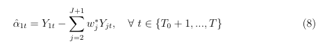
α1t = YI1t − YN1t = Y1t − YN1t                         (3)

5Whilst this region does frequently experience hurricane seasons, the hurricanes are assumed to be unpredictable because the timing, severity and affected areas is unknown. Since Y I 1t is the outcome if the county is affected by the hurricanes, the data for this is observable. This means that, in order to estimate α1t, one only needs to estimate YN 1t for t > T0, which is how the outcome variable would have evolved for the affected county absent of the hurricanes (i.e. the counterfactual).

3.3 Estimation

Suppose that Y Nit is given by a factor model:

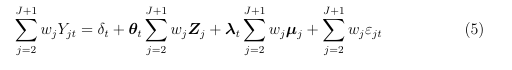
YNit = δt +θtZi +λtµi +εit

Abadie (2021) details that δt is an unknown common factor with constant factor loadings across counties, Zi is a (r × 1) vector of observed predictors of the
outcome variable (e.g. the job separation rate) that are not impacted by the hurricanes6, θt is a (1 × r) vector of unknown parameters, λt is a (1 × F) vector of unobserved common factors, µi is a (F × 1) vector of unknown factor loadings, whilst εit are the unobserved transitory outcome variable shocks at the county level with mean zero ∀ i and t. This linear factor model has some advantageous properties relative to standard difference-in-differences and fixed effects models in the sense that it allows Y N jt to depend on more than one unobserved component in
µj, with a coefficient of λt that varies across time periods. Consider a (J ×1) vector of weights W = (w2,…,wJ+1)′ where all weights and non-negative and sum to one wj ≥ 0 for j = 2,…,J +1 and w2 +···+wJ+1 = 1.
Each specific value of W represents a potential synthetic control (i.e. a specific weighted average of control counties). As a result, the value of the outcome variable 6This study only uses predictor variable data prior to the intervention so satisfies the condition that predictor variables are not affected by the hurricanes.

(e.g. the job separation rate) for each synthetic control indexed by W is given by

As a result, Abadie et al. (2010) derived an estimate of the lead specific causal effect of an intervention (the hurricane season) on the outcome variable of interest ˆ α1t. This is done by supposing that there exists a set of weights (w∗ 2,…,w∗ J+1) which satisfies {J+1 j=2 w∗ j such that the sum of weighted pre-hurricane outcome variable values for the control units will equal the pre-hurricane outcome variable values for the hurricane affected (treated) county (shown in equation 6), as well as the weighted summation of observed covariates across the control counties being equal to the observed covariates for the hurricane affected county (equation 7).

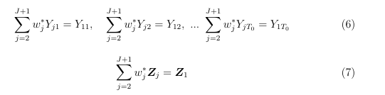
Using this, they then prove that under standard conditions, and if the quantity of pre-hurricane time periods is large compared to the scale of the unobserved shock in the outcome variable ε, the unobserved common factors λt and the unobserved shocks will be close to zero in expectation. This means that they find ˆ α1t to be a consistent estimator of α1t where

The system of equations in (6) and (7) can only hold exactly if (Y1,1,….,Y1,T0 ;Z′
1) belongs to the convex hull of sum of(Y2,1,…,Y2,T0 ;Z′ 2),….,(YJ+1,1,…,YJ+1,T0 ;Z′ J+1)}. In practice, Abadie (2021)notes that regularly there can be no set of weights that  exist which can allow these equations to hold perfectly with real world data. However, if this is the case, the synthetic control weights will be assigned such that the equations hold approximately and the researcher can check this by ensuring that the predictor variables, for the treated unit and weighted average of control units, match closely.

3.4 Computation

The outcome variable (e.g. job separation, hiring or turnover rate) is observed for
T time periods for the hurricane affected county Y1t, (t = 1,…,T) and the counties
that were not impacted by the hurricanes Yjt, (j = 2,…,J + 1;t = 1,…,T). The
quantity of post-hurricane time periods T1 can be defined as the difference between
the total time periods and the number of pre-hurricane time periods, thus
T1 = T −T0. Consider Y1 as the (T1 ×1) vector of post-hurricane outcomes for the
affected county and Y0 as the (T0 ×J) matrix of post-hurricane outcomes for the
pool of potential control counties.

Abadie et al. (2010) further defines the (T0 × 1) vector K = (k1,…,kT0 ) to be a linear combination of pre-hurricane outcomes sum ofY-K i = T0 s=1 ksYis, this means that if sumof T0−1 s=1 ks = 0 and kT0 = 1, then Y-K = YiT0 , then this will be outcome variable of interests’ value in the time period before the hurricane (i.e. 2005 Q2). Let there be M of these linear combinations, following the vectors K1,….,KM. The authors then let X1 = (Z′ 1,Y- K1 j ,…,Y KM j )′ be a (k ×1) vector of pre-hurricane characteristics for the hurricane affected county, where k =r+M. Similarly, X0 is a (k ×J) matrix which holds the same characteristics but for the potential control counties.

The optimal weighting vector W∗ is picked to minimise the gap between X1 and X0W (i.e. ∥ X1−X0W ∥), subject the conditions mentioned earlier, where weights are non-negative and sum to 1. To measure the gap between the pre-hurricane

characteristics for the affected county and the pool of potential control counties,
the weighting matrix W is often chosen to minimise

characteristics for the affected county and the pool of potential control counties,
the weighting matrix W is often chosen to minimise

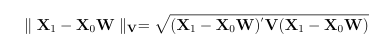
where V is defined by the authors as being a (k ×k) symmetric and positive semidefinite matrix. The choice of V influences, and is picked to minimise, the means square error of the estimator (i.e. the expectation of
(Y1 −Y0W∗)′(Y1 −Y0W∗)). However, most past comparative case studies, this paper included, choose a more data driven approach by specifying that V is picked to minimise the mean squared prediction error of the outcome variable in the pre-hurricane time periods. As such, Y K1 i1 = Yi1 ,…., YKT0 i1
=YiT0 is selected as a choice for the set of linear combinations of pre-hurricane outcomes, this is because it will include the entire pre-hurricane outcome variable sample when building the synthetic control.

3.5 Extension to Multiple Treated Units

Whilst, the original synthetic control methodology was designed with just one treated unit in mind (e.g. the Basque region in Abadie and Gardeazabal, 2003 or West Germany in Abadie et al. 2015), the methodology has since been extended to allow for studies with multiple treated units. Typically, this extension has come in two forms. The first being to compare instances where multiple units are affected by the same intervention, with the second being to compare multiple case studies where one unit is affected in each. However, these two forms are analogous because the treatment effects from one hurricane on multiple counties can also be thought of as multiple hurricanes each on one county, when estimating the average treatment effect (Cavallo et al. 2013).

As such, this study follows the approach laid out by Cavallo et al. (2013), which sought to estimate the casual impact of natural disasters on economic growth. They generalise the placebo procedure used in Abadie et al. (2010), which estimates a counterfactual for all the untreated units as well as the treated one, in
order to observe whether the treatment effect of the treated unit was notably different from the untreated ones. Here, Cavallo et al. (2013) combine the placebo effects in order to undertake inference about the average normalised effect across the unit specific comparative case studies of multiple disasters. Following Cavallo et al. (2013), the statistical command used in this study matches each county with its synthetic counterpart for the evolution of the outcome variable (e.g. the job separation, hiring or turnover rate), meaning that the estimated county-specific impact of the hurricanes is calculated as the difference between the evolution of the actual outcome variable and the evolution of its counterfactual. A result of this process is that the size of the treatment effect will depend on the size of the outcome variable for each county, therefore the estimates are normalised by
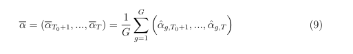
setting the outcome variable equal to one in the quarter prior to the hurricanes, to account for this scaling effect. After the estimates are normalised, the county specific results for the hurricane affected counties can be pooled to calculate the average effect of the hurricanes on the outcome variable of interest. Recall from Section 3.3, the lead-specific estimates of the hurricane season on a single affected county (indexed as county 1 earlier), was denoted as (α1,T0+1,…,α1,T) for leads 1,2,…,T − T0. Then one can calculate the average effect of the hurricanes across G counties, shown by

3.6 Inference

Abadie et al. (2010) notes that the standard errors normally shown in regression-based comparative cases studies measure the uncertainty surrounding aggregate data, yet this approach of inference would yield zero standard errors in the synthetic control methodology because aggregate data is used in estimation
procedure. Although this is not to say that there isn’t uncertainty surrounding the parameters of interest, the effect of hurricanes on the rate of labour market transitions. This is because uncertainty, related to whether the control group can reliably produce the counterfactual, remains. Cavallo et al. (2013) follows Abadie and Gardeazabal (2003) and Abadie et al. (2010) in using exact inference techniques to conduct inference within synthetic control studies. Abadie and Gardeazabal (2003) state that this is possible irrespective of the number of control units and pre-intervention periods, but the accuracy of inference grows with the quantity of control units and pre-intervention periods. This is beneficial given the 406 potential control counties used in this study, as well as the availability of quarterly data which increases the number of pre-hurricane time periods. Following the permutation tests in Abadie et al. (2010), the synthetic control methodology is applied to each of the 406 potential control counties. The purpose of this is to examine if the hurricane effect, estimated by the synthetic control procedure, for a hurricane-hit county is notably bigger than the effect estimated for a randomly selected control county. Whilst, Abadie et al. (2010) and Cavallo et al. (2013) implement one-sided permutation inference tests7, this paper conducts a two-sided variation, following Galiani and Quistorff (2017), to allow for the
possibility that our outcome variables, for example the hiring rate, may fall in the 7Both papers conduct one-sided tests as their studies are both focused on estimating the negative impact of intervention(s) on GDP per capita.

immediate aftermath of the storms, yet rise above its counterfactual in the longer term, due to the rebuilding effort. Therefore, the lead-specific significance level (p-value) for the estimated impact of the hurricanes on one treated county is given by:

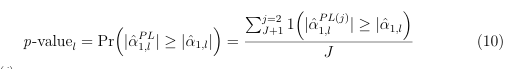
Here, ˆ αPL(j) 1,l PL(j) 1,l
denotes the l-specific effect of the hurricane season when control county j is assigned a placebo hurricane season at the same time as the affected county, it is computed using the same method as is used for ˆ α1,l. Through estimating ˆ ∀ j counties in the potential control group (J), the distribution of placebo effects can be used to examine how the estimated ˆ α1,l ranks in this distribution.

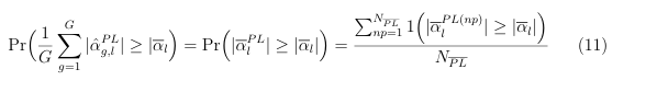
In order to modify this inference approach for multiple treated units (α), Cavallo et al. (2013) construct a distribution of average placebo effects. First, for each hurricane affected county g, all the placebo hurricane effects are estimated, thus jg = 2,3,…,Jg + 1. Then, at each lead, every possible placebo average effect is computed by selecting one placebo estimate corresponding to each county g and then taking the average across the G placebos. The number of possible placebo averages is large and is denoted by NPL. The authors then index all possible placebo averages by np = 1,2,…,NPL. Next, the lead-specific average hurricane effect for the hurricane affected counties (αl) is ranked within the entire distribution of NPL average placebo effects. Then the lead l specific p-value for the average hurricane effect across all affected counties can be computed by (11). Cavallo et al. (2013) go on to state that confidence intervals for the average hurricane effect can be constructed via the inversion of the lead-specific p-values in (11).

4 Results

Section 4 presents the results for the average impact of the 2005 Atlantic hurricane season on the job separation, hiring and turnover rates. Section 4.1 presents these results for our main specification where the treatment group is defined as those counties where at least 1% of housing units suffered severe or major damage, defined
by FEMA. Section 4.2 extends this analysis by splitting the three levels of damage (severe, major and minor) out into separate synthetic control specifications, this allows one to compare the average hurricane effect across different degrees of housing damage. Section 4.3 focuses on investigating whether there were any positive or negative spillover effects on labour market transition rates, from the hurricane season, on counties that neighboured damaged counties. Finally, Section 4.4 will explore how the hurricane effects differed by industrial sector.

4.1 Effects on Labour Market Transitions

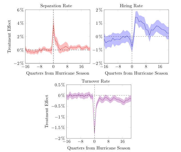
As explained in detail in Section 2.2, this paper’s main specification defines a hurricane affected county as one where at least 1% of housing units suffered damage in excess of $5,200. As a result, 63 counties are classed as the treated units, with 406 counties that neither received any damage nor neighboured damaged counties making up the control group. Following the methodology discussed in Section 3, for each outcome variable of interest (the job separation, hiring and turnover rates), a value for Y N it (i.e. the counterfactual) is estimated for each affected county from 2001 Q3 to 2010 Q4. Then the evolution of the actual outcome variable is compared to it’s synthetic counterfactual counterpart, this gap can be seen as the county-specific impact of the hurricane season. This hurricane effect is then averaged over all affected counties to derive an estimate for the average impact of the hurricanes across all affected counties. Accompanying the estimated treatment effects, period-specific 95% confidence intervals are also constructed following Cavallo et al. (2013), as explained in Section 3.6, to allow us to assess whether the estimated impact of the hurricane is statistically significant. Figure 1 below shows the average estimated gap between the actual observed labour market transition series and their synthetic counterparts, often called the treatment effect. The first point to note is that, across each of the three synthetic control models, the synthetic treatment groups closely reproduce the actual observed data in the pre-hurricane time period. This is shown through the distance between observed outcomes and their synthetic control being close to zero, and their 95% confidence intervals encompassing zero throughout the pre-hurricane period. In addition, for each of the three models in Figure 1, the synthetic control methodology also produces a comparison between the actual pre-hurricane characteristics of the affected counties (discussed in Section 2.4) and that of the
synthetic affected counties, this showed that the synthetic controls accurately reproduced the values of the labour market transition rates and their predictor variables prior to the hurricane season8. As a result, the lack of distance between the observed data and synthetic data, across predictor variables and the labour
market transition rates shown in Figure 1, suggests that the synthetic hurricane-damaged counties provide a sensible approximation for the evolution of the job separation, hiring and turnover rates that would have occurred had the 2005 Atlantic hurricane season not taken place. 8Tables presenting the pre-hurricane predictor variables and their synthetic counterparts, as well as the weights assigned to each control county by the synthetic control algorithm, do not significantly contribute to the conclusions derived from the results of this paper, thus are available upon request. This also applies for the equivalent tables in Sections 4.2, 4.3 and 4.4

Figure 1: Gap between outcomes and synthetic controls (with confidence intervals)

4.1.1 Job Separations

Figure 1 presents our estimate for the effect of the 2005 hurricane season on three labour market transition rates of interest. As is common across significant natural disasters, individuals may have become detached from their jobs for a variety of reasons. Firstly, the large number of fatalities and injuries, as a result of the storms, may have pushed some workers to leave their jobs in order to physically recover or help family member to recover, whether that be health-wise or to repair homes. Secondly, damage to one’s home may force workers to migrate to find
shelter elsewhere, meaning some workers may have been forced to leave their jobs if their new residence meant their daily commute was no longer viable. It could also be the case that physical and economic damage to businesses, such as repair costs or lower revenues resulting from a reduction in demand for their goods or services, may mean that it is no longer profitable for some businesses to stay open, either temporarily or permanently. This would result in a negative shock to labour demand and an increased likelihood of workers losing their jobs. It may have also been the case that damage to personal or public transportation, and it’s infrastructure (e.g. roads and bridges), could have prevented people showing up to their workplaces, as well as potentially disrupting the supply chains that allow businesses to operate as usual.
This paper finds that the difference between the job separation rate and its synthetic version suggests that the hurricanes caused a short-term spike in the proportion of the workforce that left their jobs. Indeed, during 2005 Q3 (when the storm season hit the US Gulf coast), the average job separation rate across the affected region rose 3.7 percentage points above its counterfactual. It is interesting to note that the confidence interval for the job separation rate only remained above zero from 2005 Q3 to 2006 Q1. This is logical given many of the mechanisms by which natural disasters can increase job separations, as explained above, are likely to have been mitigated after a few quarters (e.g. via the repair of homes, businesses and transportation infrastructure).

4.1.2 The Hiring Rate

In contrast to the impact on the separation rate, our results suggest that the job hiring rate fell marginally in the immediate aftermath of the hurricanes, but bounced back and remained notably above its counterfactual for much of the post-storm time period. As with the evolution of the job separation and turnover
rates, the path of the hiring rate will be driven by the local demand and supply of labour for each affected county, the degree of damage and the proportions of jobs that belong to different industrial sectors. Figure 1 shows that in 2005 Q3, the hiring fell by 0.75 percentage points relative to its synthetic control. This is
consistent with the notion that businesses faced significant disruption in the immediate aftermath of the storms, which may have slowed or completely stopped hiring plans for some heavily affected firms. For example, businesses may have been forced to close, or chose to divert funding from labour expenditure to capital expenditure to make physical repairs, or halted hiring plans due to increased uncertainty about future sales and revenue. However, it should also be stated that the confidence intervals indicate a statistically significant fall in the hiring rate, but that it was likely marginal, given the upper band of the confidence interval showed
a 0.3 percentage point fall in 2005 Q3. In the quarters following 2005 Q3, Figure 1 presents a significant and sustained rise in the hiring rate on average, reaching 1.5 percentage points above its synthetic control by the start of 2006. This is consistent with much of the research focusing on the impact of the storms on earnings. For example, Groen et al. (2020) show a large fall in earnings in affected areas, due to job separations, yet statistically significant evidence for higher earnings in the medium and longer-term, relative to multiple control groups. They argue that this was driven by a rise in the demand for labour during the rebuilding effort. The persistence in the elevated hiring rate, compared to the short sharp spike in the rate of job separations, likely reflects notion that, whilst hurricanes cause significant devastation across a short period of time, it can take years for communities to rebuild and recover. Groen et al. (2020) also argue that the post-2008 recession strength in earnings and employment of the hurricane hit area, relative to control areas, was driven by a quicker rebound due to the rebuilding effort, whereas control areas suffered a more prolonged slowdown after the recession. This effect may help to explain the post-recession strength of the hiring rate in affected counties.

4.1.3 Job Turnover

The final labour market variable this paper focuses on is the job turnover rate, which the US Census Bureau describe as an indicator for the degree of churn in a labour market (Abowd et al. 2006). Figure 1 shows that the job turnover rate experienced a short-term statistically significant fall of almost two percentage points on average across hurricane-hit counties. In the medium and longer-term, the storm effect on the turnover rate of damaged counties fluctuated between 0 and 0.5 percentage points below its synthetic control.
The reasoning behind the immediate fall in the quarterly job turnover rate can be partly explained with help from this paper’s results for the separation and hiring rates. Indeed, a large increase in job separations and a fall in hiring rates during 2005 Q3 are indicative of a fall in demand for labour. This means that those recently separated from jobs may find it harder to find a new job in the very short-term, relative to areas unaffected by the storm season. Furthermore, with a greater risk of job separation and lower labour demand, workers still within employment face heightened job insecurity and may have responded to this by halting or delaying plans to change jobs in the short-term. Indeed, this result is consistent with the pro cyclical nature of labour market churn and turnover. For example, Lazear and Spletzer (2012) find that job turnover declines in economic downturns as job separations rise, yet a decreasing proportion of these separations are followed by replacement hires, meanwhile workers are reluctant to quit jobs, therefore businesses slow their hiring in response.
In the medium and longer-term, the job turnover rates remains marginally below its counterfactual, with the confidence intervals suggesting that the hurricane’s effect may have been zero or close to zero in the post hurricane time period. One reason why the turnover rate may be slightly subdued in the longer-term is that
the average job may be fresher, relative to the control group. With a spike in separations in 2005 Q3 and an increase in hiring in subsequent quarters, a greater proportion of workers will be in fresh new jobs. It is certainly plausible, that the jobs gained immediately after the storm season may be associated with shorter
tenures, given workers may be less likely to wait for a job that closely matches their skills, thus are more likely to leave after a shorter period of time. However, Hyatt and Spletzer (2014) show that on average across the US, from 2005-2010, the majority of workers stay in their new job for three or more quarters. Therefore, the slightly subdued turnover rate after the initial shock may be a result of a greater proportion of workers being in new jobs, leading to less job turnover in periods after the hiring spike at the start of 2006, relative to a labour market unaffected by a storm season.

4.2 Effects by Degree of Damage

Next we can investigate whether the storm season’s impact on the evolution of labour market transition rates differed by the degree of damage that counties  suffered. As explained in Section 2.2, we assign counties into three different treatment groups. The first group is all counties where at least 1% of their housing units suffered over $30,000 in damages (severe damage group). The major damage group consists of all counties where at least 1% of housing units suffered between $5,200 and $30,000 in damages, and that these counties are not in the severe damage group. Finally, the minor damage group consists of counties who had at least 1% of housing units damaged but that these damage costs are below $5,200, and that these counties are in neither the severe or major damage groups. Here, the severe damage group consists of 19 counties, the major damage group contains 39 different counties and the minor damage group consists of 63 different counties. The group of potential control counties is the same as in Section 4.1, consisting of 406 counties that had zero damage and didn’t neighbour damaged counties. Given there are three distinct control groups, the synthetic control methodology is
carried out for each control group for each of our three labour market transition variables. This is because the 19 counties in our severe damage treatment group for example, may have very different pre-hurricane county characteristics to the 63 counties in the minor damage group, therefore the procedure is carried out
separately for each treatment group to ensure that the estimated counterfactuals provide good approximations for each individual damage group. As a result, it should be clear that, with three distinct treatment groups and three outcomes variables, this section of the paper involves three separate synthetic control estimations to be carried out per outcome variable. Then for each outcome variable and degree of damage, the hurricane effect is again calculated as the average difference between the observed evolution of that specific series and its estimated counterfactual. Figure 2 presents the results for the effect the hurricane season had on the separation, hiring and turnover rates, split by the level of damage inflicted.

Figure 2: Gap between Outcome and Synthetic Controls by Degree of Damage

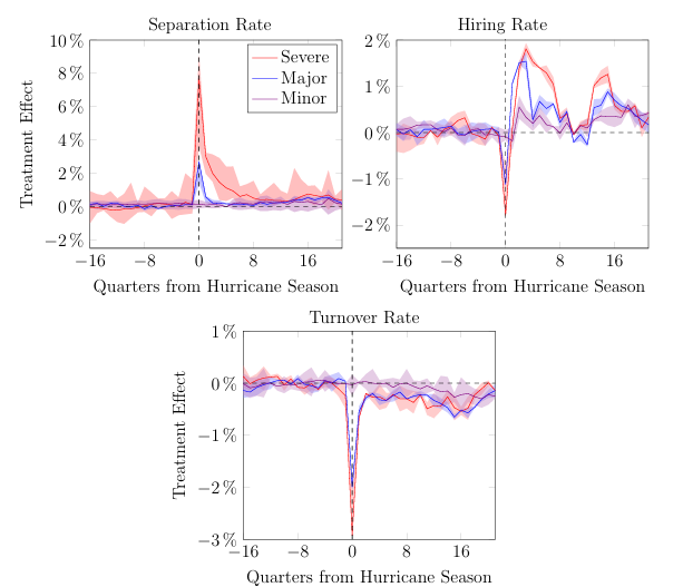
Naturally, it’s clear that counties suffering severe damage saw a much larger average rise in the job separation rate than majorly and marginally damaged counties, relative to their respective counterfactuals. The mechanisms behind how hurricanes can cause a rise in the separation rate, discussed in Section 4.1.1, are likely to be amplified when examining the results for severely damaged counties, compared to  the majorly and marginally damaged counties. A significant reason for this is that many of the severely damaged counties had much higher incidences of long-term evacuation, due to flooding, 40% of these long-term evacuees never returned to
their pre-storm residences and this increased the likelihood of job losses, relative to residents who didn’t evacuate or those who could return to the same residence after evacuating (Vigdor, 2007). The results from the synthetic control procedures carried out show close matching in the pre-storm period across damage degrees,
then a statistically significant average rise of almost 8 percentage points for the job separation rate for severely damaged counties. Meanwhile, majorly damaged counties showed a smaller, but still significant, rise of almost 2.5 percentage points.

The impact on majorly damaged counties was also noticeably less persistent than that seen for severely damaged counties, with the effect becoming statistically indistinguishable from zero by 2006 Q1 compared to this occurring for the severe damage group by 2007 Q1. There was no evidence of an elevated average job separation rate amongst counties that suffered minor storm damage. Regarding the impact the storm season had on the job hiring rate, results shown in Figure 2 suggest the magnitude of change was much smaller than changes in the job separation, echoing the results in Section 4.1. Again, severely damaged counties experienced larger average changes, relative to majorly damaged counties. Here, severely damaged counties suffered a statistically significant fall of almost 2 percentage points in 2005 Q3 but rose to be above its counterfactual by a similar magnitude by 2006 Q2. The results for the minor damage group showed that some of the post-storm hurricane average impact on the hiring rate were statistically insignificant at times, and when significant, were relatively small, but do show some indication of benefiting from the labour shortages and the post-recession bounce back seen in affected areas towards the end of our sample.  Similarly, the turnover rate shows a larger fall on average for severely damaged counties than majorly damaged counties, with marginally damaged counties showing little to no statistical decrease in the average turnover rate. This suggests that the hypothesis of a spike separations and subsequent rise in hiring afterwards, causing a greater proportion of fresher jobs and thus lower turnover, discussed in Section 4.1.3., appears driven by severely and majorly damaged counties. Whilst few existing studies look at the impact of the 2005 storms on labour market variables by the degree of damage suffered, this paper’s findings appear consistent with the conclusions made by past studies. For example, Groen at al. (2020) also estimate the storm effects separately by degree of housing damage, they find earnings losses associated with severe and major damage to be greatest. Their findings show earnings losses lasted for roughly two years which is notably longer than the persistence this paper finds for the evolution of the separation rate. However, this may reflect the idea that, since Groen et al. (2020) estimate that 97% of short-term earnings losses were a result of separations, separations in the immediate aftermath of the storms can weigh heavily on an individual’s earnings in subsequent quarters, even once the storms’ effect on the separation rate has dissipated. As a result, we would expect greater persistence in changes in quarterly earnings than changes in quarterly separations. Groen et al. (2020) also show that the earnings of individuals suffering minor damage outperformed majorly damaged earnings, this could partly be explained by the lack of noticeable job separations amongst the minor damage group of counties in this study.

4.3 Spillover Effects

This section will explore whether the damage generated in hurricane-hit counties impacted the evolution of labour market transitions in neighbouring counties that suffered no damage. This area of analysis can be justified on the basis that if the negative labour market impacts of the storm season leech out into neighbouring
counties, then policymakers should take this into account when allocating aid. Spillover effects from natural disasters are typically split into two groups, the spillover effects from the disaster itself and the spillover effects in the longer-term recovery period. Whilst there is typically less focus on the spillover effects than the direct effects of natural disasters, there are multiple instances where evidence of spillover effects has been found. For example, Seetharam (2018) estimated that for every manufacturing job lost in a US hurricane-affected county, an additional 0.19 to 0.25 manufacturing jobs are lost in unaffected counties for multi-plant firms, driven by resource constraints and managerial distraction. Furthermore, Kates et al. (2006) summarise how the US Great Plains droughts in the 1890s, the Mississippi floods in 1927, and the dust bowl droughts in the 1930s, all led to large negative economic effects for nearby areas that were not impacted by the droughts or floods, this was primarily due to outward migration. Indeed, there are multiple possible mechanisms by which hurricane effects could manifest in neighbouring counties. Firstly, with an elevated rate of job separation amongst affected counties, adjacent counties could experience an influx of labour supply which could result in an increased hiring rate, if labour shortages were present or businesses could expand quickly. Secondly, the economic harm to households and firms in affected counties may result in lower incomes and potentially less spending in neighbouring counties if shoppers frequently spend across county lines, less spending in neighbouring counties could result in more job separations or subdued hiring in these unaffected counties. It could also be the case that if many businesses were forced to close temporarily or permanently, consumer and firm spending may be diverted away from affected counties and towards neighbouring counties, thus could result in positive labour market outcomes. In the longer-term, one can also consider that the disaster recovery funding could also positively spillover into adjacent counties, furthermore the population of unaffected nearby counties may benefit from the job opportunities related to the building effort in affected areas, especially construction workers.

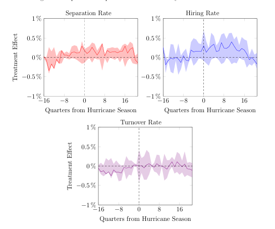
To investigate whether there was evidence of spillovers at the aggregate level, this section defines the treated group as any county that suffered no hurricane damage according to HUD (2006), but geographically neighbours at least one county that did suffer damage. In our sample there were seven such counties. The same
synthetic control methodology is applied as before, following Section 3, for each of our three labour market transition rates. As shown in Figure 3, this paper fails to find conclusive evidence of statistically significant average storm effects across the job separation, hiring and turnover rates. Here, the 95% confidence intervals
encompass zero hurricane effect across the entire post-storm time period. It should be noted that it may be the case that there are multiple opposing spillover effects that balance for each county in the treatment group. Alternatively, there may be evidence of spillovers in the treated counties but when the effects are averaged across the seven counties, following the Cavallo et al. (2013) extension for multiple treated units, the overall storm effects are indistinguishable from zero.

Figure 3: Gap between Spillover Outcomes and Synthetic Controls

4.4 Hurricane Effects by Industrial Sector

This section seeks to extend the results presented in Section 4.1 by exploring whether the storm season’s effects on labour market transition rates differed across industrial sectors. Understanding how workers moved around the labour market, by industry, has important implications for policymakers who seek to target disaster relief packages to workers most affected. For example, given the results from research discussed earlier, which stated that 97% of short-term earnings decreases were driven by job separations, understanding where an elevated risk of job separation is likely to occur, can help policymakers mitigate the effects of disasters for affected populations. In order to understand how the storm effects varied by industry, this paper exploits
the industrial sector cuts of labour market transition data in the Quarterly Workforce Indicators, rather than using the industry aggregated QWI data like in Sections 4.1, 4.2 and 4.3. Here the treatment group is defined as in Section 4.1, where counties that had at least 1% of housing units experiencing damage costs of $5,200 or greater were classed as treated. As in all other sections of this paper, the potential control group is defined as any county that suffered no damage, did not neighbour any damaged counties, and was in a state that had at least one county experiencing damage from the 2005 Atlantic hurricane season, thus 406 counties are
available to be used as possible controls. Storm effects are considered across the Agriculture & Natural Resources, Construction, Manufacturing, Trade & Transport, Education & Healthcare, Utilities, Professional Services, and Accommodation & Leisure industrial sectors. The synthetic control procedure is
carried out separately for each industrial sector, for each of the three labour market transition rates in this study.
The hurricane effects are presented in Figure 4 as the difference between the observed labour market transition rate for a given sector and the estimated counterfactual for that sectoral labour market transition rate.Figure 4 shows that the impacts of the storms on labour market transitions were, to a degree, heterogeneous across industrial sectors. The greatest magnitude of impact was felt in the construction sector (shown in red) and the accommodation and leisure sector (shown in blue).

Figure 4: Gap between Outcomes and Synthetic Controls by Industrial Sector

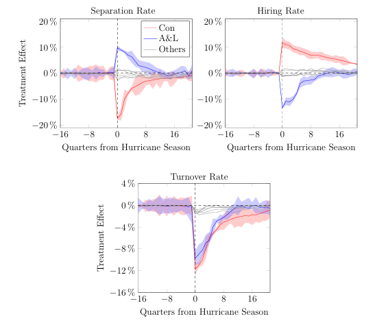
Here we can see that the job separation rate in the construction sector dropped over 17 percentage points in 2005 Q3, in contrast, the separation rate in the accommodation and leisure sector rose by almost 10 percentage points. The results for these two sectors appears consistent with the existing findings on the impact of the hurricane season on labour market outcomes by industry. Indeed, Groen et al. (2020) find evidence for increased demand for construction services related to the post-hurricane rebuilding effort, they found that wages in the construction sector rose by 4.8% in the immediate aftermath and 22.7% by the end of this paper’s sample. Therefore, a large and statistically significant fall in quarterly average job separations amongst hurricane-affected counties follows the evidence in industry earnings dynamics.

The inverse effect holds true for the accommodation and leisure industry. Here, Groen et al. (2020) estimate a 8.5% fall in earnings in the short-term, they also state that these earnings losses persisted into the medium term. Therefore, our results, suggesting a significant rise in the average job separation rate in this sector,
appears consistent with the notion that social consumption and tourism was greatly disrupted by the storms. A report from the Louisiana Recovery Authority (2006) found that 1,409 tourism and hospitality businesses shut down completely due to the storms, affecting 33,000 hospitality-based employees in Louisiana alone.
The findings for the storm seasons’ impact on the other six industries (all shown in grey) found more modest impacts, which were not statistically significant. This is interesting in the sense that Groen et al. (2020) estimated that wages fell significantly (-9.3%) in the healthcare sector, tradable sectors related to the rebuilding effort such as agriculture & resources and manufacturing saw large positive earnings effects, whilst our analysis found that labour market transitions in these sectors didn’t change significantly. This suggests that wage changes in these
sectors may have primarily been driven by within employment earnings changes rather than earnings changes as a result of separations and hirings. The results for the effects on the job separation rate can be traced back to the industry aggregate results in Figure 1. This is because whilst the fall in the separation rate is larger in construction than in accommodation and leisure, Table 1 shows that the latter comprises a larger share of the economy than the construction sector, in the treated
counties. Therefore, the rise in separations from the accommodation and leisure industry appear to dominate the fall in separations from the construction sector. Due to this, and the insignificant effects for industries with larger sectoral weightings, the aggregate industry effect is a rise, of much smaller magnitude, in the overall separation rate.

When studying how the hiring rate evolved for different industries, it is clear that a similar and logical narrative begins to emerge. This is because, in both existing literature and our results for the separation rate, the construction sector appears to have largely benefited from the storm season, whilst the accommodation and leisure sector suffered greatly. This is also shown in the hiring rate across industries in Figure 4, where the hiring rate in the construction sector rose by almost 12 percentage points, meanwhile the hiring rate in the accommodation and leisure sector fell by 13 percentage points in the immediate aftermath of the storm season. Given the other six industries studied didn’t show any statistically significant hurricane effects in the separation rate, it is not surprising that our results also show no significant effect in the hiring rate for these industries.

One interesting point to note is that the hiring rate in the construction sector remains above its respective counterfactual and is significant across the entire post-hurricane sample, meanwhile storm effects on the hiring rate for the accommodation and leisure sector only persist until 2008 Q2. This may partially explain why the industry-aggregated hiring rate in Figure 1 remains largely above its counterfactual in the medium and longer term. Another possible explanation for this may be that the accommodation and leisure industry is often regarded as having relatively fewer job requirements for new workers and this sector generally has a high turnover of staff. Therefore, it may be the case that whilst hiring fell more sharply in this sector, it was able to rebound to its counterfactual hiring rate quicker than the construction sector.

Estimates in Figure 4 show that the hurricane season resulted in a significant decrease in the job turnover rate across the construction and accommodation and leisure industries. In 2005 Q3, the turnover rate in the construction sector was 12 percentage points below its counterfactual, whilst this rate for the leisure and
accommodation fell 10 percentage points relative to its synthetic counterpart. As with the separation and hiring rates, the results showed no significant storm effects on the turnover rate of the six other industries studied. Comparing these results to Figure 1, it is clear that the two sectors of interest drove much of the aggregate fall
in the turnover rate, whilst relatively minor falls amongst other sectors resulted in an aggregate fall of much smaller magnitude. Results from Figure 4 also suggest that much of the mostly significant below counterfactual fluctuations in the turnover rate, shown in Figure 1, may have been driven by subdued turnover in the
construction sector rather than the accommodation and leisure sector, or other sectors. This is likely because of the elevated demand for construction labour required in the rebuilding effort, leading to large earnings growth as detailed by Groen et al. (2020), thus potentially fewer incentives for construction works to change jobs, resulting in lower job turnover in the sector.

5 Conclusion

This study contributes to our knowledge on how labour market outcomes are affected by natural disasters by investigating the extent to which labour market transitions changed as a result of the 2005 Atlantic hurricane season. We find that, amongst hurricane-affected counties, the average job separation rate rose
significantly and the job turnover rate fell in the immediate aftermath of the storm. Meanwhile, the hiring rate fell initially, before increasing well above a weighted average of control counties in subsequent quarters. These results were consistent with the relevant literature on the evolution of earnings and employment after the storm season. We show that there was a clear relationship between the severity of housing damage suffered and the change in labour market transition rates observed. Here, counties with increasingly severe damage experienced larger increases in job separations, more significant changes in hiring, and bigger declines in the job turnover rate.

This paper also explored whether any impact of the storm season could be detected in the labour market transitions of undamaged neighbouring counties. However, the estimates for the average storm effects showed no evidence of aggregate spillovers across county lines. Breaking down the impact that the hurricane season had on labour market movements by industry, we are able to show that the construction
(positively) and accommodation and leisure (negatively) sectors were most affected. These findings support and add context to previous research which show the hurricanes had heterogeneous effects across industries for labour market outcomes. The conclusions derived from these results demonstrate the importance in policymakers considering targeted disaster responses. Indeed, it appears economic assistance for the accommodation and leisure industry could be most beneficial on preventing job separations, thus reducing the likelihood of large declines in the earnings path of workers in this sector. Putting the results into a broader context, it should also be recognised that, given the scale of destruction, the quarterly impact of the storms on worker transitions was relatively small in the long-term. This provides a more detailed backdrop to the wealth of research that suggests that the incomes of storm-affected people significantly surpassed matched control groups in the long-term (e.g. Elliot and Pais, 2006; Dolfman et al. 2007; Belasen and Polachek, 2008; Zissimopoulos and Karoly, 2010; Sisk and Bankston, 2014; Gallagher and Hartley, 2017; Boustan et al. 2017; Deryugina et al. 2018; Groen et al. 2020).

This study adds to the body of literature on the impact of the 2005 Atlantic hurricane season on labour market outcomes in a number of ways. Firstly, Deryugina et al. (2018) and Groen et al. (2020) are the only other papers to analyse outcomes across a significant post-hurricane time horizon, albeit they focus on wages and employment rather than labour market transitions. To the best of our knowledge, this paper is the first to study such transitions, in relation to the 2005 storms. This paper, along with Groen et al. (2020), are the only causal inference papers to study the evolution of labour market outcomes across all affected counties, rather than a specific city, region or state.

Whilst this paper explores four interesting avenues relating to the storm season, this research could be improved or extended. Firstly, the use of alternative control groups, such as county data from alternative US states, could allow us to conclude that the estimated storm affects are robust across a variety of different control
groups. Secondly, the analysis only focuses on whether spillover effects are present in neighbouring undamaged counties, whilst there is justification for this, the approach could be extended by examining whether spillover effects were present in large cities. This would be motivated by the findings of McIntosh (2008) and De Silva et al. (2010) who show evidence of changes in labour market outcomes in Houston as a result of hurricane-induced migration. Attempts to separate out the competing mechanisms in which spillover can occur, rather than studying a rather opaque aggregated average effect, would also significantly improve this research.

Other such possible avenues for related future research include the estimation of the proportion of separated workers that were re-hired to the same job, given the large but short-term spike in separations. One could also look at the rate of job-to-job flows as an alternative to the three outcomes discussed in this paper. There is also an opportunity to enhance the empirical framework used, Abadie (2021) notes that the process of dividing the pre-intervention period, into a training and validation period, can result in improved pre-intervention matching of the treated and control groups.

6 References

Abadie , A. and L’Hour, J. (2021), “A penalized synthetic control estimator for
disaggregated data.” Journal of the American Statistical Association, 116(536), pp.
1817-34.
Abadie, A. (2021). “Using synthetic controls: Feasibility, data requirements, and
methodological aspects”. Journal of Economic Literature, 59(2), pp. 391-425.
Abadie, A. and Gardeazabal, J. (2003). “The economic costs of conflict: A case
study of the Basque Country.” American Economic Review, 93(1), pp. 113-132.
Abadie, A. and Vives-i-Bastida, J. (forthcoming). “Synthetic Controls in Action.”
Econometric Society Monographs.
Abadie, A., Diamond, A. and Hainmueller, J. (2010). “Synthetic control methods
for comparative case studies: Estimating the effect of California’s tobacco control
program.” Journal of the American Statistical Association, 105(490), pp. 493-505.
Abadie, A., Diamond, A. and Hainmueller, J. (2015). “Comparative Politics and
the Synthetic Control Method.” American Journal of Political Science, 59(2), pp.
495–510.
Abowd, J., Stephens, B, Vilhuber, L., Andersson, F., McKinney, K.L., Roemer, M.
and Woodcock, S. (2006). “The LEHD Infrastructure Files and the Creation of the
Quarterly Workforce Indicators.” Longitudinal Employer-Household Dynamics
Technical Papers, 2006-01, Centre for Economic Studies, U.S. Census Bureau.

Belasen, A.R. and Polachek, S.W. (2008). “How hurricanes affect wages and
employment in local labor markets.” American Economic Review, 98(2), pp. 49–53.
Black, E.S., Landsea, C. and Gibney, E.J. (2011) The deadliest, costliest, and most
intense United States tropical cyclones from 1851 to 2010 (and other frequently
requested hurricane facts). National Hurricane Centre. Miami, Florida.
Boustan, L.P., Kahn, M.E., Rhode, P.W. and Yanguas, M.L. (2017). “The effect of
natural disasters on economic activity in US counties: A century of data. NBER
Working Paper no. 23410, National Bureau of Economic Research, Cambridge, MA.
Card, D. (1990). ”The Impact of the Mariel Boatlift on the Miami Labor
Market.“ ILR Review, 43(2), pp. 245-57.
Card, D. and Krueger, A.B. (1994). ”Minimum Wages and Employment: A Case
Study of the Fast Food Industry in New Jersey and Pennsylvania.” American
Economic Review, 84(4), pp. 772-93.
Cavallo, E., S. Galiani, I. Noy, and J. Pantano. (2013). “Catastrophic natural
disasters and economic growth”. Review of Economics and Statistics, 95(5), pp.
1549–1561.
Clayton, R.L. and Spletzer, J.R. (2006). “Worker mobility before and after
Hurricane Katrina.” Monthly Labor Review, 129(8), pp. 11–21.
Coffman, M. and Noy, I. (2012). “Hurricane Iniki: Measuring the long-term
economic impact of a natural disaster using synthetic control.” Environment and
Development Economics, 17(2), pp. 187–205.

De Silva, D.G., McComb, R.P., Young-Kyu, M., Schiller, A.R. and Vargas, A.J.
(2010). “The effect of migration on wages: Evidence from a natural experiment.”
American Economic Review, 100(2), pp. 321–26.
Deryugina, T., Kawano, L. and Levitt, S. (2018). “The economic impact of
Hurricane Katrina on its victims: Evidence from individual tax returns.” American
Economic Journal: Applied Economics, 10(2), 202–233.
Dolfman, M.L., Wasser, S.F. and Bergman, B. (2007). “The effects of Hurricane
Katrina on the New Orleans economy.” Monthly Labor Review, 130(3), pp. 3–18.
Dube, A. and Zipperer, B. (2015). “Pooling Multiple Case Studies Using Synthetic
Controls: An Application to Minimum Wage Policies.” IZA Discussion Paper, 8944.
Elliott, J.R. and Pais, J. (2006). “Race, class, and Hurricane Katrina: Social
differences in human response to disaster.” Social Science Research, 35(2), pp.
295–321.
Galiani, S. and Quistorff, B. (2017). “The synth runner package: Utilities to
automate Synthetic Control Estimation using Synth.” Stata Journal, 17(4), pp.
834-849.
Groen, J,A. and Polivka, A.E. (2008). “The Effect of Hurricane Katrina on the
Labor Market Outcomes of Evacuees.” American Economic Review, 98(2), pp.
43-48.
Groen, J.A., Kutzbach, M.J. and Polivka, A.E. (2020). “Storms and Jobs: The
Effect of Hurricanes on Individuals’ Employment and Earnings over the Long
Term.” Journal of Labour Economics, 38(3), pp. 653-85.

Hainmueller, J. (2012). “Entropy Balancing for Causal Effects: A Multivariate
Re-weighting Method to Produce Balanced Samples in Observational Studies.”
Political Analysis, 20(1), pp. 25-46.
HUD (US Department of Housing and Urban Development). (2006). “Current
housing unit damage estimates: Hurricanes Katrina, Rita, and Wilma.”
Washington, DC: Office of Policy Development and Research, HUD.
Hyatt, H.R and Spletzer, J.R. (2014) ”Hires, Separations, And The Job Tenure
Distribution In Administrative Earnings Records,“ Working Papers 14-29, Center
for Economic Studies, U.S. Census Bureau.
Kates, R.W., Colten, C.E., Laska, S. and Leatherman, S.P. (2006).
”Reconstruction of New Orleans after Hurricane Katrina: A research
perspective.“ Proceedings of the National Academy of the Sciences of the Unites
States of America, 103(40), 14653-14660.
Kletzer, L.G. (1998). “Job Displacement.” Journal of Economic Perspectives,
12(1), pp. 115–36.
Knabb, R.D., Brown, D.P. and Rhome, J.R. (2005) Tropical cyclone report:
Hurricane Katrina. National Hurricane Centre. Miami, Florida.
Lazear, E. and Spletzer, J. (2012). “Hiring, Churn, and the Business Cycle,”
American Economic Review Papers and Proceedings, 102(3), pp. 575-579.
Louisiana Recovery Authority. (2006). Proposed Action Plan Amendment Number
2 for Disaster Recovery Funds Disaster Recovery Initiative. Baton Rouge: Office of
Community Development.

McIntosh, M.F. (2008). “Measuring the labor market impacts of Hurricane Katrina
migration: Evidence from Houston, Texas.” American Economic Review, 98(2), pp.
54–57.
National Oceanic and Atmospheric Administration. (2006). State of the Climate:
Hurricanes and Tropical Storms– Annual 2005. National Centers for Environment
Information. Hancock, Mississippi.
Robbins, M.., Saunders, J. and Kilmer, J. (2017). “A Framework for Synthetic
Control Methods with High-Dimensional, Micro-Level Data: Evaluating a
Neighborhood-Specific Crime Intervention.” Journal of the American Statistical
Association, 112(517), pp. 109–26.
Sacerdote, B. (2012). “When the saints go marching out: Long-term outcomes for
student evacuees from Hurricanes Katrina and Rita.” American Economic Journal:
Applied Economics, 4(1), pp. 109–35.
Seetharam, I. (2018). “The indirect effects of hurricanes: Evidence from firm
internal networks.” Stanford Working Paper.
Sisk, B. and Bankston III, C.L. (2014). “Hurricane Katrina, a construction boom,
and a new labor force: Latino immigrants and the New Orleans construction
industry, 2000 and 2006–2010.” Population Research and Policy Review, 33(3), pp.
309–34.
Vigdor, J.L. (2008). “The economic aftermath of Hurricane Katrina.” Journal of
Economic Perspectives, 22(4), pp. 135–54.

Vigdor, J.L. (2008). “The Katrina Effect: Was There a Bright Side to the
Evacuation of Greater New Orleans?” NBER Working Papers 13022, National
Bureau of Economic Research, Inc.
Zissimopoulos, J. and Karoly, L. (2010). “Employment and self-employment in the
wake of Hurricane Katrina.” Demography, 47(2), pp. 345–67.

7 Appendix

Table 1 below presents summary statistics, as discussed in Section 2.4. It shows the average pre-hurricane (2001 Q3 to 2005 Q2) value for each variable used in the main specification of this paper, carried out in Section 4.1. This is shown for both the treatment and control groups.